Take-home EX1

Take-home Exercise 1: Geospatial Analytics for Social Good

Setting the Scene

Water is an important resource to mankind. Clean and accessible water is critical to human health. It provides a healthy environment, a sustainable economy, reduces poverty and ensures peace and security. Yet over 40% of the global population does not have access to sufficient clean water. By 2025, 1.8 billion people will be living in countries or regions with absolute water scarcity, according to UN-Water. The lack of water poses a major threat to several sectors, including food security. Agriculture uses about 70% of the world’s accessible freshwater.

Developing countries are most affected by water shortages and poor water quality. Up to 80% of illnesses in the developing world are linked to inadequate water and sanitation. Despite technological advancement, providing clean water to the rural community is still a major development issues in many countries globally, especially countries in the Africa continent.

To address the issue of providing clean and sustainable water supply to the rural community, a global Water Point Data Exchange (WPdx) project has been initiated. The main aim of this initiative is to collect water point related data from rural areas at the water point or small water scheme level and share the data via WPdx Data Repository, a cloud-based data library. What is so special of this project is that data are collected based on WPDx Data Standard.

Objectives

Geospatial analytics hold tremendous potential to address complex problems facing society. In this study, you are tasked to apply appropriate global and local measures of spatial Association techniques to reveals the spatial patterns of Not Functional water points. For the purpose of this study, Nigeria will be used as the study country.

The Data

Apstial data

For the purpose of this assignment, data from WPdx Global Data Repositories will be used. There are two versions of the data. They are: WPdx-Basic and WPdx+. You are required to use WPdx+ data set.

Geospatial data

Nigeria Level-2 Administrative Boundary (also known as Local Government Area) polygon features GIS data will be used in this take-home exercise. The data can be downloaded either from The Humanitarian Data Exchange portal or geoBoundaries.

Getting Started

In the code chunk below, p_load() of pacman package is used to install and load the following R packages into R environment:

sf: used for importing, managing and processing geospatial data

tidyverse: a set of packages for data science

tmap: used to generate thematic maps

spdep: used to create spatial weights matrix objects

funModeling: used for rapid Exploratory Data Analysis

pacman::p_load(sf, tidyverse, tmap, spdep, funModeling)

Importing Geospatial Data

In this in-class data, two geospatial data sets will be used, they are:

geo_export
nga_admbnda_adm2_osgof_20190417

Importing water point geospatial data

First, we are going to import the water point geospatial data (i.e. geo_export) by using the code chunk below.

wp <- st_read(dsn="geodata",
              layer="geo_export",
              crs=4326) %>%
  filter(clean_coun == "Nigeria")

Next, write_rds() of readr package is used to save the extracted sf data table (i.e. wp) into an output file in rds data format. The output file is called wp_nga.rds and it is saved in geodata sub-folder.

wp_nga <- write_rds(wp,
                    "geodata/wp_nga.rds")

Importing Nigeria LGA boundary data

nga <- st_read(dsn="geodata",layer="nga_admbnda_adm2_osgof_20190417",
               crs=4326)

Data Wrangling

Recoding NA values into string

replace_na() is used to recode all the NA values in status_cle field into Unknown.

wp_nga <- read_rds("geodata/wp_nga.rds") %>%
  mutate(status_cle = replace_na(status_cle, "Unknown"))

EDA

freq() of funModeling package is used to display the distribution of status_cle field in wp_nga.

freq (data=wp_nga,
      input = "status_cle")

There are 9 different status of data, for the convenience of analysis, we will group them into 3 categories.

Functional: Functional, Functional but needs repair, Functional but not in use.

Non functional: Non-Functional, Non-Functional due to dry season, Non functional due to dry season, Abandoned

Unknown: Unknown

Extracting funtional water point

wpt_functional <- wp_nga %>%
  filter(status_cle %in%
           c("Functional", 
             "Functional but not in use",
             "Functional but needs repair"))
freq(data=wpt_functional, input="status_cle")

freq(data=wpt_functional, 
     input = 'status_cle')

Extracting non-funtional water point

wpt_nonfunctional <- wp_nga %>%
  filter(status_cle %in%
           c("Abandoned/Decommissioned", 
             "Abandoned",
             "Non-Functional",
             "Non functional due to dry season",
             "Non-Functional due to dry season"))

freq(data=wpt_nonfunctional, 
     input = 'status_cle')

Extracting water point with Unknown class

wpt_unknown <- wp_nga %>%
  filter(status_cle == "Unknown")

Performing Point-in-Polygon Count

nga_wp <- nga %>% 
  mutate(`total wpt` = lengths(
    st_intersects(nga, wp_nga))) %>%
  mutate(`wpt functional` = lengths(
    st_intersects(nga, wpt_functional))) %>%
  mutate(`wpt non-functional` = lengths(
    st_intersects(nga, wpt_nonfunctional))) %>%
  mutate(`wpt unknown` = lengths(
    st_intersects(nga, wpt_unknown)))

Saving the Analytical Data Table

nga_wp <- nga_wp %>%
  mutate(pct_functional = `wpt functional`/`total wpt`) %>%
  mutate(`pct_non-functional` = `wpt non-functional`/`total wpt`) %>%
  select(3:4, 9:10, 18:23)

Now, we have the tidy sf data table subsequent analysis. We will save the sf data table into rds format.

write_rds(nga_wp, "geodata/nga_wp.rds")

Visualising the spatial dsitribution of water points

nga_wp <- read_rds("geodata/nga_wp.rds")
total <- qtm(nga_wp, "total wpt")
wp_functional <- qtm(nga_wp, "wpt functional")
wp_nonfunctional <- qtm(nga_wp, "wpt non-functional")
unknown <- qtm(nga_wp, "wpt unknown")

tmap_arrange(total, wp_functional, wp_nonfunctional, unknown, asp=1, ncol=2)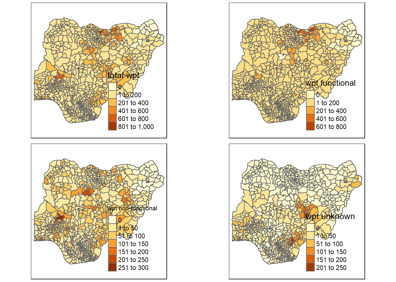

st_crs(nga_wp)

Coordinate Reference System:
  User input: EPSG:4326 
  wkt:
GEOGCRS["WGS 84",
    ENSEMBLE["World Geodetic System 1984 ensemble",
        MEMBER["World Geodetic System 1984 (Transit)"],
        MEMBER["World Geodetic System 1984 (G730)"],
        MEMBER["World Geodetic System 1984 (G873)"],
        MEMBER["World Geodetic System 1984 (G1150)"],
        MEMBER["World Geodetic System 1984 (G1674)"],
        MEMBER["World Geodetic System 1984 (G1762)"],
        MEMBER["World Geodetic System 1984 (G2139)"],
        ELLIPSOID["WGS 84",6378137,298.257223563,
            LENGTHUNIT["metre",1]],
        ENSEMBLEACCURACY[2.0]],
    PRIMEM["Greenwich",0,
        ANGLEUNIT["degree",0.0174532925199433]],
    CS[ellipsoidal,2],
        AXIS["geodetic latitude (Lat)",north,
            ORDER[1],
            ANGLEUNIT["degree",0.0174532925199433]],
        AXIS["geodetic longitude (Lon)",east,
            ORDER[2],
            ANGLEUNIT["degree",0.0174532925199433]],
    USAGE[
        SCOPE["Horizontal component of 3D system."],
        AREA["World."],
        BBOX[-90,-180,90,180]],
    ID["EPSG",4326]]

Visualising Regional Development Indicator

equal <- tm_shape(nga_wp) +
  tm_fill("wpt non-functional",
          n = 5,
          style = "equal") +
  tm_borders(alpha = 0.5) +
  tm_layout(main.title = "Equal interval classification")

quantile <- tm_shape(nga_wp) +
  tm_fill("wpt non-functional",
          n = 5,
          style = "quantile") +
  tm_borders(alpha = 0.5) +
  tm_layout(main.title = "Equal quantile classification")

tmap_arrange(equal, 
             quantile, 
             asp=1, 
             ncol=2)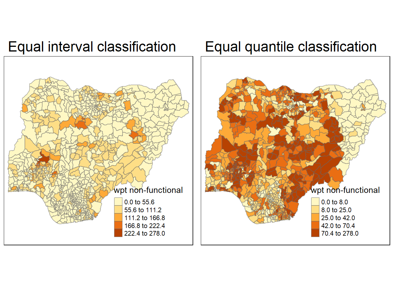

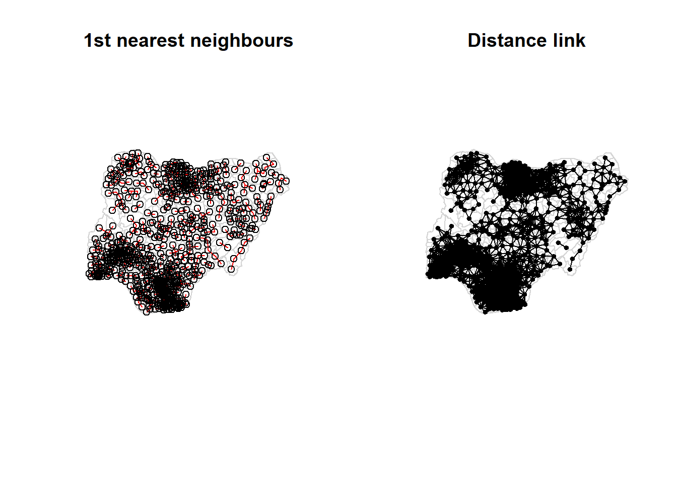
To ensure the consistency of the analysis scale, the fixed distance method will be used. Determine the centroid for each area

coords <- st_centroid(st_geometry(nga_wp))

Determine the cutoff distance for fixed distance weight matrix

k1 <- knn2nb(knearneigh(coords))
k1dists <- unlist(nbdists(k1, coords))
summary(k1dists)

   Min. 1st Qu.  Median    Mean 3rd Qu.    Max. 
  2.675  12.814  20.300  22.075  27.800  72.027

The result shows that the maximum distance is 72.027.

threshold <- max(unlist(nbdists(k1, coords)))

Computing Fixed distance weight matrix

wm_d73 <- dnearneigh(coords, 0, threshold)
wm_d73

Neighbour list object:
Number of regions: 774 
Number of nonzero links: 18050 
Percentage nonzero weights: 3.012973 
Average number of links: 23.32041

Each region have average 23 neighbors.

Visualizing the Distance weight Matrix

par(mfrow=c(1,2))
plot(nga_wp$geometry, border="lightgrey", main="1st nearest neighbours")
plot(k1, coords, add=TRUE, col="red", length=0.08)
plot(nga_wp$geometry, border="lightgrey", main="Distance link")
plot(wm_d73, coords, add=TRUE, pch = 19, cex = 0.6)

Assigning weights to each neighboring polygon

wm73_lw <- nb2listw(wm_d73, 
                   style="W", 
                   zero.policy = TRUE)
summary (wm73_lw )

Characteristics of weights list object:
Neighbour list object:
Number of regions: 774 
Number of nonzero links: 18050 
Percentage nonzero weights: 3.012973 
Average number of links: 23.32041 
Link number distribution:

 1  2  3  4  5  6  7  8  9 10 11 12 13 14 15 16 17 18 19 20 21 22 23 24 25 26 
 5  8 12 21 34 33 33 37 28 34 28 20 19 22 15 13 13 16 12 15 16 13 11 11  6 14 
27 28 29 30 31 32 33 34 35 36 37 38 39 40 41 42 43 44 45 46 47 48 49 50 51 52 
10  5 14 14 13  7  9  9 11  9 11 14 13 11  9  5  3  5  6  9  8  9  4  5  3  3 
53 54 55 56 57 58 59 60 61 62 63 64 65 67 68 
 2  4  5  4  6  5  2  5  5 10  7  3  3  4  1 
5 least connected regions:
90 112 123 237 670 with 1 link
1 most connected region:
585 with 68 links

Weights style: W 
Weights constants summary:
    n     nn  S0       S1       S2
W 774 599076 774 130.1845 3126.732

The weight of the first polygon’s neighbors

wm73_lw$weights[10]

[[1]]
 [1] 0.01587302 0.01587302 0.01587302 0.01587302 0.01587302 0.01587302
 [7] 0.01587302 0.01587302 0.01587302 0.01587302 0.01587302 0.01587302
[13] 0.01587302 0.01587302 0.01587302 0.01587302 0.01587302 0.01587302
[19] 0.01587302 0.01587302 0.01587302 0.01587302 0.01587302 0.01587302
[25] 0.01587302 0.01587302 0.01587302 0.01587302 0.01587302 0.01587302
[31] 0.01587302 0.01587302 0.01587302 0.01587302 0.01587302 0.01587302
[37] 0.01587302 0.01587302 0.01587302 0.01587302 0.01587302 0.01587302
[43] 0.01587302 0.01587302 0.01587302 0.01587302 0.01587302 0.01587302
[49] 0.01587302 0.01587302 0.01587302 0.01587302 0.01587302 0.01587302
[55] 0.01587302 0.01587302 0.01587302 0.01587302 0.01587302 0.01587302
[61] 0.01587302 0.01587302 0.01587302

Using Moran’s | for Global Spatial Autocorrelation

moran.test(nga_wp$`wpt non-functional`, 
           listw=wm73_lw, 
           zero.policy = TRUE, 
           na.action=na.omit)


    Moran I test under randomisation

data:  nga_wp$`wpt non-functional`  
weights: wm73_lw    

Moran I statistic standard deviate = 22.517, p-value < 2.2e-16
alternative hypothesis: greater
sample estimates:
Moran I statistic       Expectation          Variance 
     0.3273418398     -0.0012936611      0.0002130078

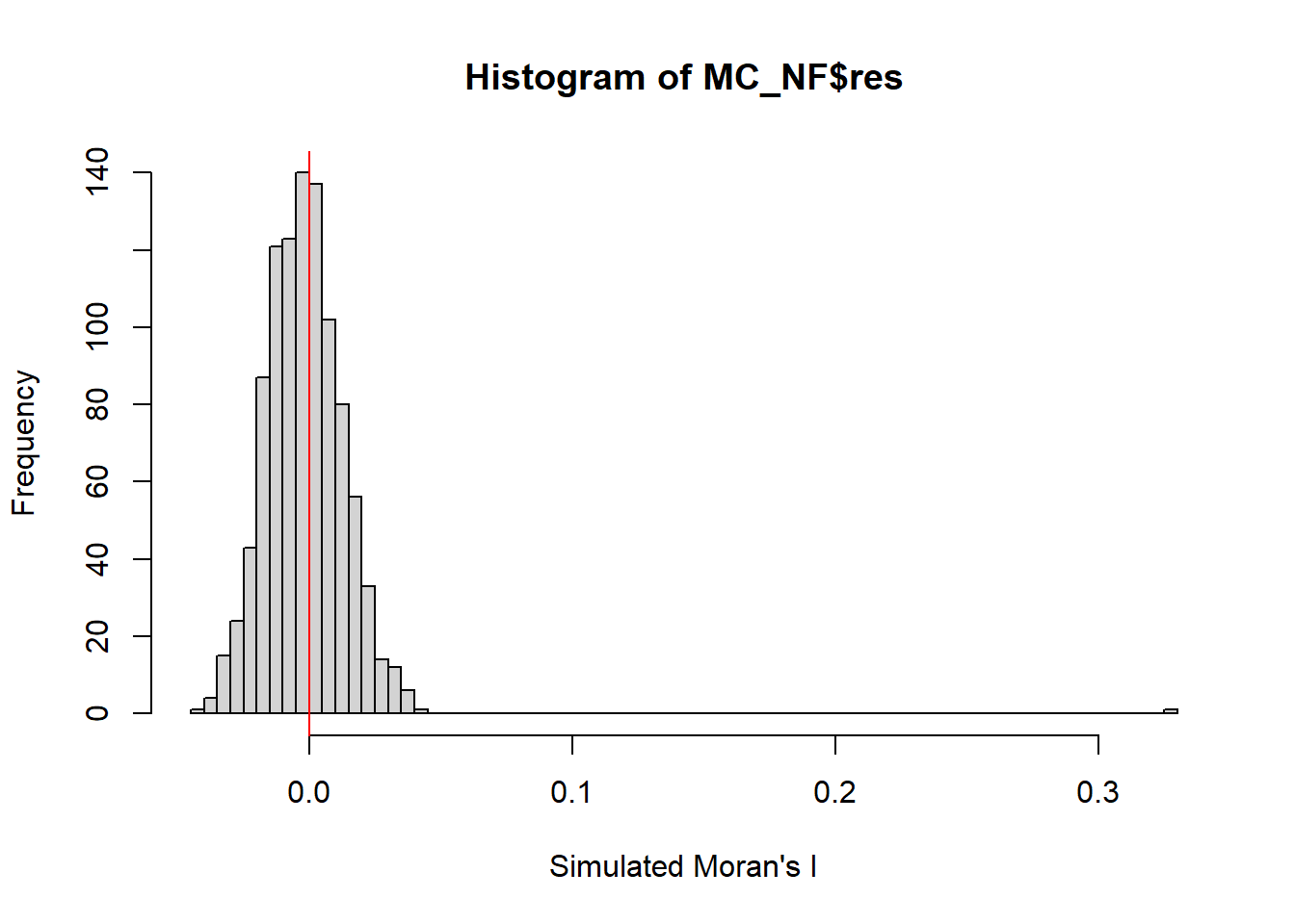
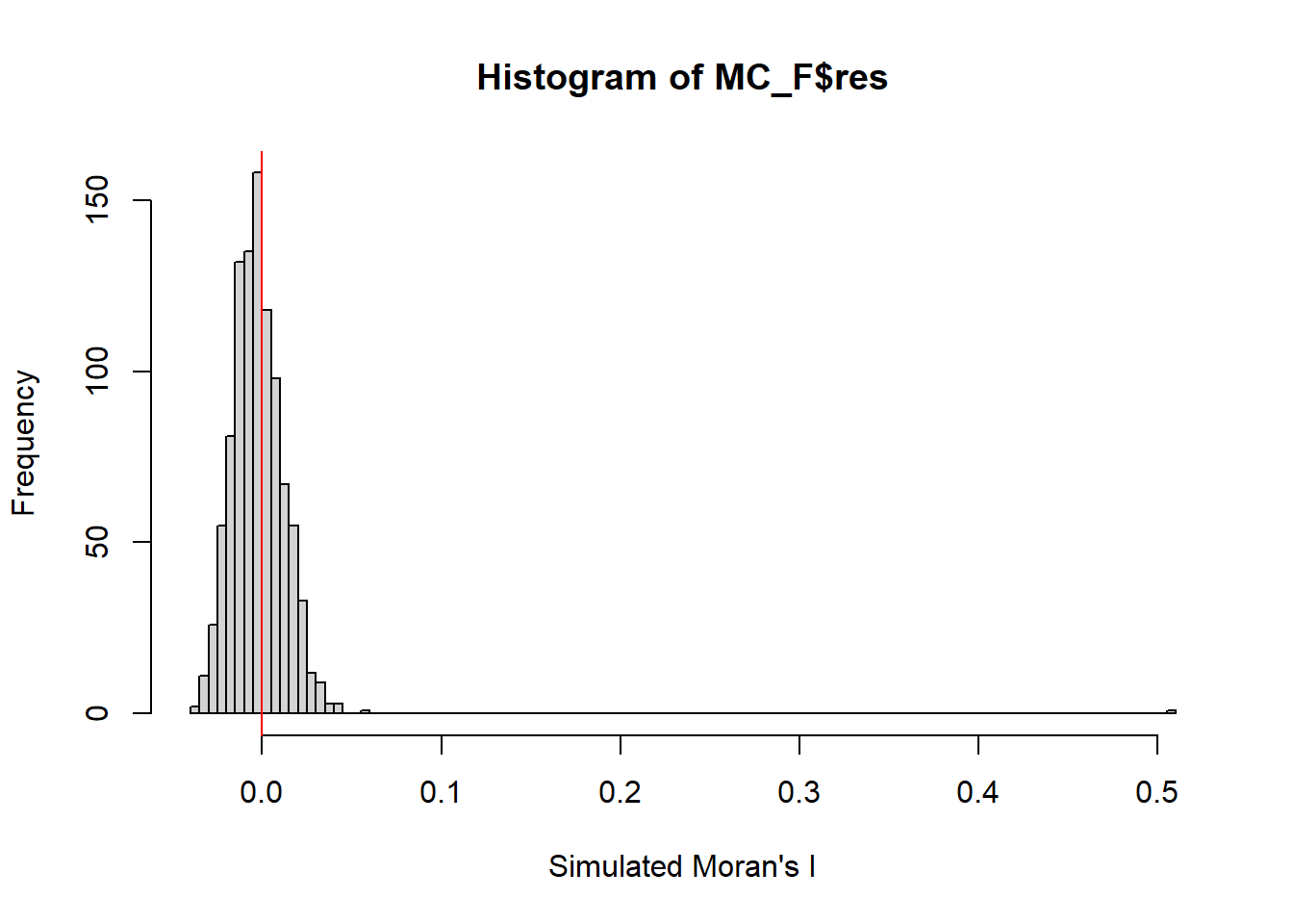
Computing Monte Carlo Moran’s |

set.seed(1234)
MC_NF= moran.mc(nga_wp$`wpt non-functional`, 
                listw=wm73_lw, 
                nsim=999, 
                zero.policy = TRUE, 
                na.action=na.omit)
MC_NF


    Monte-Carlo simulation of Moran I

data:  nga_wp$`wpt non-functional` 
weights: wm73_lw  
number of simulations + 1: 1000 

statistic = 0.32734, observed rank = 1000, p-value = 0.001
alternative hypothesis: greater

set.seed(1234)
MC_F= moran.mc(nga_wp$`wpt functional`, 
                listw=wm73_lw, 
                nsim=999, 
                zero.policy = TRUE, 
                na.action=na.omit)
MC_F


    Monte-Carlo simulation of Moran I

data:  nga_wp$`wpt functional` 
weights: wm73_lw  
number of simulations + 1: 1000 

statistic = 0.50517, observed rank = 1000, p-value = 0.001
alternative hypothesis: greater

From the result Moran | value is > 0,the overall spatial autocorrelation tend to be similarly clustered. The p value is 0.001 which is statically significant. Therefore, null hypothesis should be rejected. There is sign of clustering.

Visualising Monte Carlo simulation of Moran’s |

hist(MC_NF$res, 
     freq=TRUE, 
     breaks=100, 
     xlab="Simulated Moran's I")
abline(v=0, 
       col="red")

hist(MC_F$res, 
     freq=TRUE, 
     breaks=100, 
     xlab="Simulated Moran's I")
abline(v=0, 
       col="red")

Cluster and Outlier Analysis

fips <- order(nga_wp$ADM2_EN)
localMI_dw <- localmoran(nga_wp$`wpt non-functional`, wm73_lw)
localMI_dw_FUN <- localmoran(nga_wp$`wpt functional`, wm73_lw)

head(localMI_dw_FUN)

          Ii          E.Ii      Var.Ii      Z.Ii Pr(z != E(Ii))
1 0.43151603 -7.191834e-04 0.008120236 4.7966255   1.613609e-06
2 0.27475350 -2.904635e-04 0.003338620 4.7601280   1.934703e-06
3 0.69235062 -8.956670e-04 0.345864093 1.1787856   2.384836e-01
4 0.05590525 -3.884365e-04 0.029702941 0.3266329   7.439455e-01
5 0.33277612 -3.884365e-04 0.004984321 4.7190630   2.369335e-06
6 0.05909213 -4.231402e-05 0.001519106 1.5172126   1.292130e-01

nga_wp.localMI <- cbind(nga_wp,localMI_dw) %>%
  rename(Pr.Ii.nf = Pr.z....E.Ii..)
nga_wp.localMI <- cbind(nga_wp.localMI,localMI_dw_FUN) %>%
  rename(Pr.Ii.f = Pr.z....E.Ii..)

Mapping local Moran’s I value

Moran_NF <- tm_shape(nga_wp.localMI) + 
  tm_fill("white") +
  tm_borders("grey", lwd = 0.5, alpha = 0.5) +
  tm_shape(nga_wp.localMI[nga_wp.localMI$Pr.Ii.nf <= 0.05,]) +
  tm_fill(col = "Ii", 
          style = "pretty",
          palette = "RdBu",
          title = "local moran statistics") +
  tm_borders(alpha = 0.5) +
  tm_layout(main.title = "Local Moran I value for p < 0.05 (Non Functional)",
            main.title.size = 0.7,
            main.title.fontface = "bold",
            title = "Fixed Distance Weight",
            title.size = 0.6,
            legend.height = 0.25,
            legend.width = 0.35)
  

Moran_F <- tm_shape(nga_wp.localMI) + 
  tm_fill("white") +
  tm_borders("grey", lwd = 0.5, alpha = 0.5) +
  tm_shape(nga_wp.localMI[nga_wp.localMI$Pr.Ii.f <= 0.05,]) +
  tm_fill(col = "Ii.1", 
          style = "pretty",
          palette = "RdBu",
          title = "local moran statistics") +
  tm_borders(alpha = 0.5) +
  tm_layout(main.title = "Local Moran I value for p < 0.05 (Functional)",
            main.title.size = 0.7,
            main.title.fontface = "bold",
            title = "Fixed Distance Weight",
            title.size = 0.6,
            legend.height = 0.25,
            legend.width = 0.35)

tmap_arrange(Moran_NF, Moran_F, asp = 1, ncol = 2)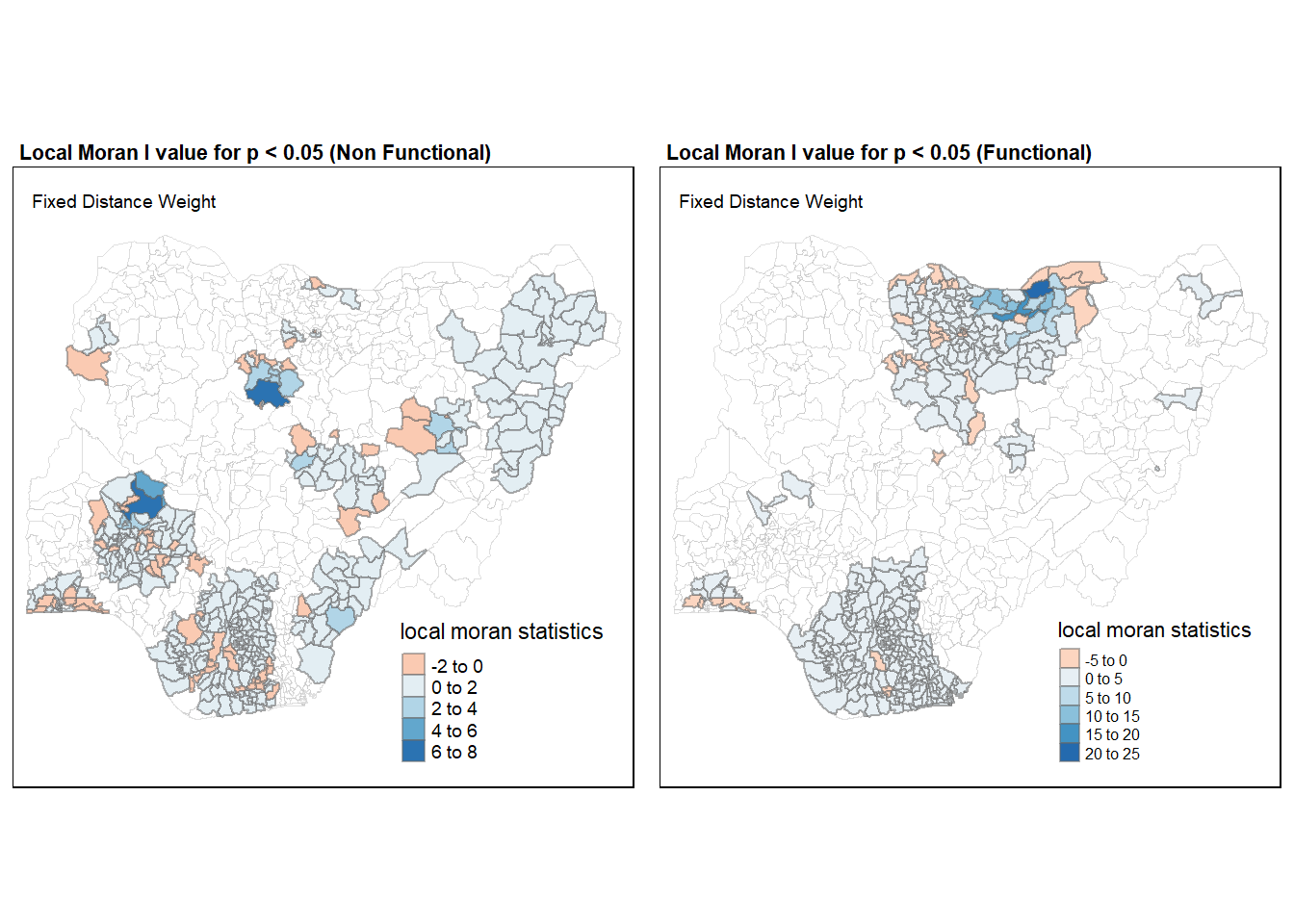

Mapping local Moran’s I p-values

p_value_nf <- tm_shape(nga_wp.localMI) +
  tm_fill(col = "Pr.Ii.nf", 
          breaks=c(-Inf, 0.001, 0.01, 0.05, 0.1, Inf),
          palette="-Blues",
          title = "local Moran's I p-values") +
  tm_borders(alpha = 0.5) +
  tm_layout(main.title = "P-value (Non-Functional)",
            main.title.size = 0.7,
            main.title.fontface = "bold",
            title = "Fixed Distance Weight",
            title.size = 0.6,
            legend.height = 0.25,
            legend.width = 0.35)


p_value_f <- tm_shape(nga_wp.localMI) +
  tm_fill(col = "Pr.Ii.f", 
          breaks=c(-Inf, 0.001, 0.01, 0.05, 0.1, Inf),
          palette="-Greens",
          title = "local Moran's I p-values" ) +
  tm_borders(alpha = 0.5) +
  tm_layout(main.title = "P-value (Functional)",
            main.title.size = 0.7,
            main.title.fontface = "bold",
            title = "Fixed Distance Weight",
            title.size = 0.6,
            legend.height = 0.25,
            legend.width = 0.35)

tmap_arrange(p_value_nf, p_value_f, asp=1, ncol=2)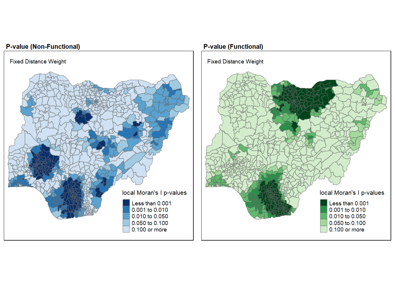

pacman::p_load(sf,tidyverse,tmap,spdep,funModeling)

Importing Geospatial Data

Importing water point geospatial data

wp <- st_read(dsn="geodata",
              layer="geo_export",
              crs=4326) %>%
  filter(clean_coun == "Nigeria")

Mapping both local Moran’s I values and p-values

Moran_NF <- tm_shape(nga_wp.localMI) + 
  tm_fill("white") +
  tm_borders("grey", lwd = 0.5, alpha = 0.5) +
  tm_shape(nga_wp.localMI[nga_wp.localMI$Pr.Ii.nf <= 0.05,]) +
  tm_fill(col = "Ii", 
          style = "pretty",
          palette = "RdBu",
          title = "local moran statistics") +
  tm_borders(alpha = 0.5) +
  tm_layout(main.title = "Local Moran I value for p < 0.05 (Non Functional)",
            main.title.size = 0.7,
            main.title.fontface = "bold",
            title = "Fixed Distance Weight",
            title.size = 0.6,
            legend.height = 0.25,
            legend.width = 0.35)
  

Moran_F <- tm_shape(nga_wp.localMI) + 
  tm_fill("white") +
  tm_borders("grey", lwd = 0.5, alpha = 0.5) +
  tm_shape(nga_wp.localMI[nga_wp.localMI$Pr.Ii.f <= 0.05,]) +
  tm_fill(col = "Ii.1", 
          style = "pretty",
          palette = "RdBu",
          title = "local moran statistics") +
  tm_borders(alpha = 0.5) +
  tm_layout(main.title = "Local Moran I value for p < 0.05 (Functional)",
            main.title.size = 0.7,
            main.title.fontface = "bold",
            title = "Fixed Distance Weight",
            title.size = 0.6,
            legend.height = 0.25,
            legend.width = 0.35)

p_value_nf <- tm_shape(nga_wp.localMI) +
  tm_fill(col = "Pr.Ii.nf", 
          breaks=c(-Inf, 0.001, 0.01, 0.05, 0.1, Inf),
          palette="-Blues",
          title = "local Moran's I p-values") +
  tm_borders(alpha = 0.5) +
  tm_layout(main.title = "P-value (Non-Functional)",
            main.title.size = 0.7,
            main.title.fontface = "bold",
            title = "Fixed Distance Weight",
            title.size = 0.6,
            legend.height = 0.25,
            legend.width = 0.35)


p_value_f <- tm_shape(nga_wp.localMI) +
  tm_fill(col = "Pr.Ii.f", 
          breaks=c(-Inf, 0.001, 0.01, 0.05, 0.1, Inf),
          palette="-Greens",
          title = "local Moran's I p-values" ) +
  tm_borders(alpha = 0.5) +
  tm_layout(main.title = "P-value (Functional)",
            main.title.size = 0.7,
            main.title.fontface = "bold",
            title = "Fixed Distance Weight",
            title.size = 0.6,
            legend.height = 0.25,
            legend.width = 0.35)
tmap_arrange(Moran_NF, Moran_F, p_value_nf, p_value_f, asp=1, ncol=2)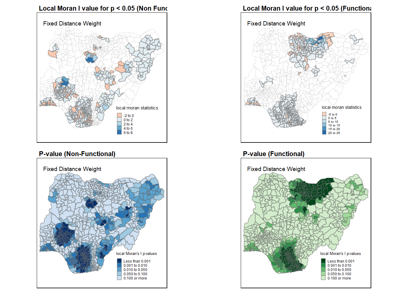

LISA Cluster Map

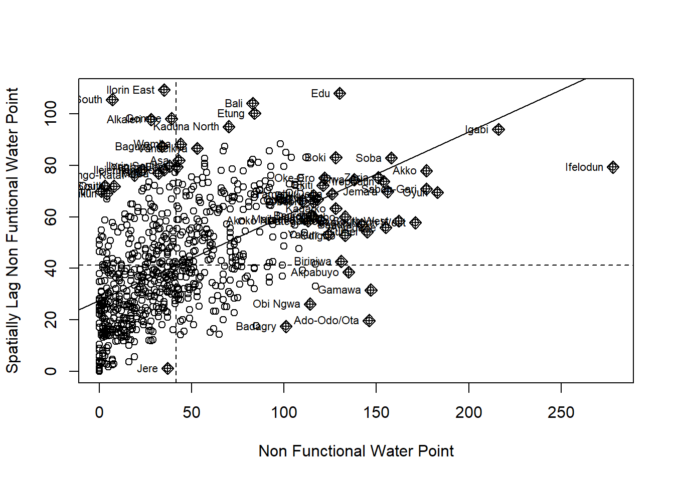
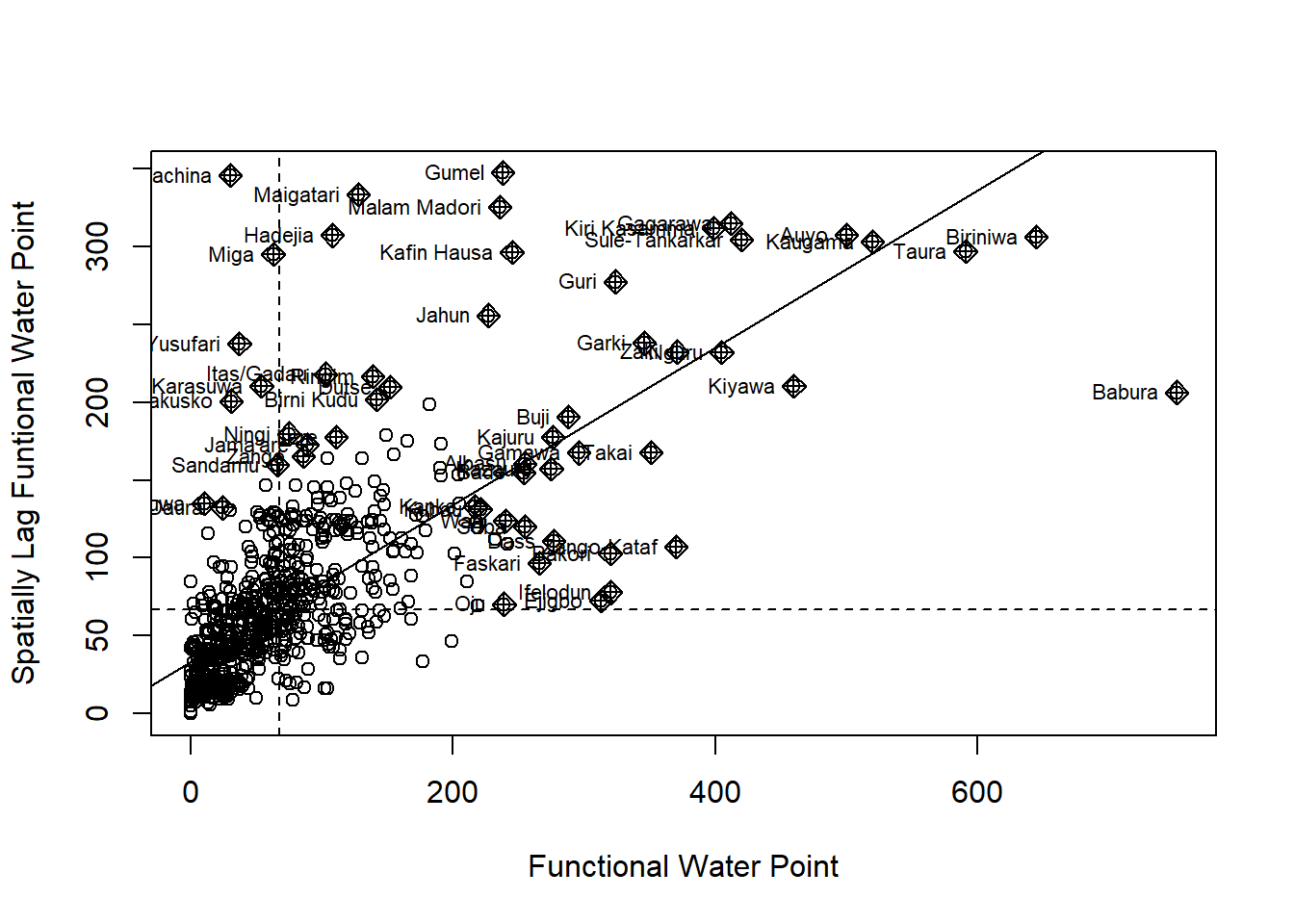
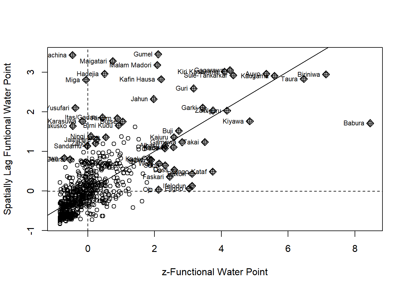
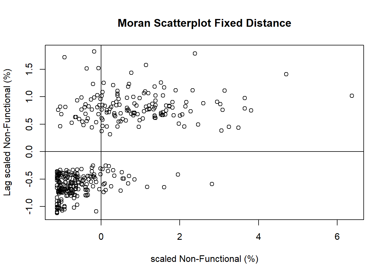
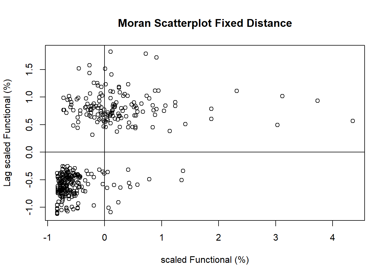
Plotting Moran scatterplot

nci <- moran.plot(nga_wp$`wpt non-functional`, wm73_lw,
                  labels=as.character(nga_wp$ADM2_EN), 
                  xlab="Non Functional Water Point", 
                  ylab="Spatially Lag Non Funtional Water Point")

nci1 <- moran.plot(nga_wp$`wpt functional`, wm73_lw,
                  labels=as.character(nga_wp$ADM2_EN), 
                  xlab="Functional Water Point", 
                  ylab="Spatially Lag Funtional Water Point")

Preparing LISA map classes

nga_wp$Z.nonfunc <- scale(nga_wp$`wpt non-functional`) %>% 
  as.vector 
nga_wp$Z.Func <- scale(nga_wp$`wpt functional`)%>%
  as.vector

nci2 <- moran.plot(nga_wp$Z.nonfunc, wm73_lw,
                   labels=as.character(nga_wp$ADM2_EN),
                   xlab="z-Non-functional Water Point", 
                   ylab="Spatially Lag z-Non-functional Water Point")

nci3 <- moran.plot(nga_wp$Z.Fun, wm73_lw,
                  labels=as.character(nga_wp$ADM2_EN), 
                  xlab="z-Functional Water Point", 
                  ylab="Spatially Lag Funtional Water Point")

quadrant <- vector(mode="numeric",length=nrow(localMI_dw))

quadrant2 <- vector(mode="numeric",length=nrow(localMI_dw_FUN))

scale waterpoint

DV <- scale(nga_wp.localMI$wpt.non.functional)
DV_Fun <- scale(nga_wp.localMI$wpt.functional)

C_mI <- lag.listw(wm73_lw, DV)
C_mI_Fun <- lag.listw(wm73_lw, DV_Fun)

Filter all the area with p-value<0.05 and identify significant areas.

MIplot <- data.frame(cbind(DV,C_mI,localMI_dw[,5]))
MIplot <- MIplot %>%
  filter (X3 < 0.05)
plot(x = MIplot$X1, y = MIplot$X2, main = "Moran Scatterplot Fixed Distance", xlab = "scaled Non-Functional (%)", ylab = "Lag scaled Non-Functional (%)")
abline(h = 0, v = 0)

MIplot <- data.frame(cbind(DV_Fun,C_mI,localMI_dw[,5]))
MIplot <- MIplot %>%
  filter (X3 < 0.05)
plot(x = MIplot$X1, y = MIplot$X2, main = "Moran Scatterplot Fixed Distance", xlab = "scaled Functional (%)", ylab = "Lag scaled Functional (%)")
abline(h = 0, v = 0)

Take-home Exercise 1: Geospatial Analytics for Social Good

Setting the Scene

Objectives

The Data

Apstial data

Geospatial data

Getting Started

Importing Geospatial Data

Importing water point geospatial data

Importing Nigeria LGA boundary data

Data Wrangling

Recoding NA values into string

EDA

Extracting funtional water point

Extracting non-funtional water point

Extracting water point with Unknown class

Performing Point-in-Polygon Count

Saving the Analytical Data Table

Visualising the spatial dsitribution of water points

Visualising Regional Development Indicator

Determine the cutoff distance for fixed distance weight matrix

Computing Fixed distance weight matrix

Visualizing the Distance weight Matrix

Assigning weights to each neighboring polygon

The weight of the first polygon’s neighbors

Using Moran’s | for Global Spatial Autocorrelation

Visualising Monte Carlo simulation of Moran’s |

Cluster and Outlier Analysis

Mapping local Moran’s I value

Mapping local Moran’s I p-values

Importing Geospatial Data

Mapping both local Moran’s I values and p-values

LISA Cluster Map

Plotting Moran scatterplot

Preparing LISA map classes

scale waterpoint

THE END